Hail Seaborn!

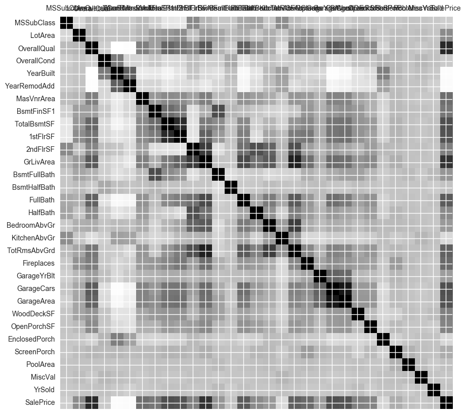
The seaborn heatmap perhaps is the best visualization of the correlations in a data set.

 Much better than Axes.matshow():

Analyzing Predictions to find *bugs*

Testing should be one of the most frequent steps in the SDLC for any code, whether it is building a website, powering a smart device or machine learning. Tests of machine learning code may reveal lots of issues - transformations that don't work because the right columns are not operated on or data which fails assumptions of the learning algorithm. The list may be endless and we are well attuned to this process. One of the tests often ignored is comparing the test results during the training period with actual values from the data and then trying to find what went wrong and where. This can often reveal attributes or column values that you may have ignored till now and must play a bigger role.

For example, use the following function to plot test results against the real values. The plot should be a straight line. Any deviations from it are to be analyzed for every column.

Make your test data comply with training data

When using scikit-learn libraries with pandas, you would often get errors if the test data does not have columns which match the model created from the training data set. You may have deleted columns that you did not need from the training data when creating the model or you may have constructed new columns based on existing data variables (for example, creating 'Age' from 'Date' or combining the effects of multiple variables). In most cases, this is simple to achieve by wringing the test data through the same function as the training data. However, when you are using One-Hot-Encoding of categorical data, the columns created as a result of this coding in the training set and the test set may not match for the simple reason that some values for categorical data may only be present in the training data set and others may be present only in the test data set. I have included here a python function that I wrote and works really well to match the test data with the training data:

K-Means Cluster Analysis on Outlook on Life Survey Data

The Outlook on Life Survey (OOL) was designed to study political and social attitudes in the United States. The project included two surveys fielded between August and December 2012 using a sample from an Internet panel. A total of 2,294 respondents participated in this study during Wave 1 and 1,601 were interviewed during Wave 2. There are 436 variables in this study.

Note that full access to data archive is available for members on the ICPSR site.

Our goal in this study is to do a K-Means Cluster Analysis to determine if there is a set of variables we can identify that can measure how angry people feel about the way things are going in the country these days (W1_B4).

The variables we selected as the cluster variables are:

Variable	Description
W1_H1	Society has reached the point where Blacks and Whites have equal opportunities for achievement
W1_O5	[Black people should teach their children to be careful around the police] How much emphasis or de-emphasis should Black people place on each statement in the education of their children?
PPINCIMP	Household Income
W1_F4_D	[To become wealthy ] For yourself and people like you, how easy or hard is it to reach these goals?
W1_F6	How far along the road to your American Dream do you think you will ultimately get on a 10-point scale where 1 is not far at all and 10 nearly there?
W1_M5	How often do you attend religious services?

We are going to validate our clusters by excluding the variable W1_B4 (Description - Generally speaking, how angry do you feel about the way things are going in the country these days?) from our analysis. We would treat this variable as a measure and we expect to see some differences on this variable amongst our clusters.

While doing the cluster analysis we noticed the following: (a) In some cases, when more data was included for determining the clusters or the cluster analysis was repeated, we observed that the cluster means for our measure variable came quite close. In addition, if the number of clusters we wanted was increased, that also had an impact on the cluster means and the significance of the difference amongst the cluster means.

First, we ran a simulation trying to determine what the affect of clustering on the average distance of the points from centroids. For our analysis, we will go with three clusters. As we can see the choice of number of clusters is completely subjective. As the number of clusters increase, the average distance will decrease.

Here is the plot of the cluster after applying PCA to reduce the number of variable dimensions to two:

The split amongst the three clusters is (the cluster IDs are 0.0, 1.0 and 2.0)

0.0    419

2.0    355

1.0    348

Our next step is to try and fit a simple least squares line using W1_B4 as the dependent variable based on the cluster number we have determined for the points. The results of that are:

The mean and standard deviation for W1_B4 in the three clusters are:

cluster        
0.0      2.916468
1.0      3.129310
2.0      3.008451
standard deviations for W1_B4 by cluster
            W1_B4
cluster        
0.0      1.307026
1.0      1.192171
2.0      1.224716

Because we had more than two clusters, we decided to conduct a tukey test to determine which one of the two means had significant difference. It seems that cluster 0.0 and cluster 1.0 had means that were significantly different (led to rejection of the null hypothesis).

Then we analyzed the two clusters are the means of the different cluster variables within those clusters.

The following is the mean of the various clustering variables in their respective clusters:

W1_B4 mean is lower for cluster 0.0 indicating that people in cluster 0.0 are generally more angry about the situation in the country than those in cluster 1.0 (lower values in the survey correspond to higher anger felt by the respondent). Then we try to look deeper into the cluster variable means. We find that W1_F4_D is lower for cluster 0.0. Lower value indicates that the respondents think that it is hard to become wealthy in this country. A lower value of W1_H1 (in cluster 0.0) indicates that the respondents agree much more that blacks and whites have equal opportunities for achievement. A lower value of W1_M5 for cluster 0.0 also indicates that respondents attend religious services more frequently there. A higher value for W1_05 for cluster 0.0 indicates that respondents place a strong emphasis that black people should teach their children to be careful around the police in the education of their children. Cluster 0.0 also has lower average household income.

So what can we establish - it seems that the likelihood that a person is going to be unhappy about the situation in this country is going to be higher when their income is lower and they generally do not believe that their wealth can significantly increase in this country (even though they believe that blacks and whites have equal opportunities). The higher likelihood seems connected with lower income, more religious bent of mind and general wariness of law enforcement.

The code is included below:

Lasso Regression for U.S. National Epidemiological Survey on Alcohol and Related Conditions (NESARC) data

Background on the data used here (NESARC) was described in an earlier post in this blog. In that post, we conducted a Random Forest analysis for the boolean response variable: EVER GAMBLED 5+ TIMES IN ANY ONE YEAR (S12Q1). In this post we conduct Lasso Regression for the same. Before we dive into the analysis, there were some interesting observations about using Lasso, which performs linear regression for a response variable. When this response variable has an integer value vs a boolean we get different results. When we use a boolean variable, the results are quite similar to the Random Forest analysis which also used a boolean response variable. However, if we use an integer value for the response variable, which makes more sense to use in a linear regression (e.g Lasso where MSE is calculated), the list of important variables detected are different from those reported by Random Forest. This requires more analysis.

The following variables (listed below in order of importance) were identified as the most important since their coefficients were the largest in absolute values in this regression. We can compare the coefficients since we scaled the input variables to zero mean and unit variance. The most important variables identified in this analysis were: whether the individual had panic attacks (S6Q1) or was engaged in reckless driving (S11AQ1A15) or was not too open with anyone including those close to him/her (S10Q1A3). The rest of the variables are mentioned as well. The variables whose coefficient was reported to be zero by Lasso are briefly mentioned below as well.

Variable	Description	Coefficients
S6Q1	HAD PANIC ATTACK, SUDDENLY FELT FRIGHTENED/OVERWHELMED/NERVOUS AS IF IN GREAT DANGER BUT WERE NOT	0.226163
S11AQ1A15	EVER GET MORE THAN 3 TICKETS FOR RECKLESS/CARELESS DRIVING, SPEEDING, OR CAUSING AN ACCIDENT	0.175727
S10Q1A3	FIND IT HARD TO BE "OPEN" EVEN WITH PEOPLE YOU ARE CLOSE TO	0.125577
S11AQ1A25	EVER DO SOMETHING YOU COULD HAVE BEEN ARRESTED FOR, REGARDLESS OF WHETHER YOU WERE CAUGHT OR NOT	0.085541
S11AQ1A2	EVER STAY OUT LATE AT NIGHT EVEN THOUGH PARENTS TOLD YOU TO STAY HOME	0.068325
S11AQ1A22	EVER SHOPLIFT	0.067515
S11AQ1A1	OFTEN CUT CLASS, NOT GO TO CLASS OR GO TO SCHOOL AND LEAVE WITHOUT PERMISSION	0.067146
S11AQ1A14	EVER DO THINGS THAT COULD EASILY HAVE HURT YOU OR SOMEONE ELSE, LIKE SPEEDING OR DRIVING AFTER HAVING TOO MUCH TO DRINK	0.054445
S9Q1A	EVER HAD 6+ MONTH PERIOD FELT TENSE/NERVOUS/WORRIED MOST OF TIME	0.047805
S10Q1A16	THE KIND OF PERSON WHO FOCUSES ON DETAILS/ORDER/ORGANIZATION OR LIKES TO MAKE LISTS AND SCHEDULES	0.047434
S1Q1G	NUMBER OF YEARS LIVED IN UNITED STATES	-0.030454
SMOKER	TOBACCO USE STATUS	0.026548
S11BQ1	BLOOD/NATURAL FATHER EVER HAD BEHAVIOR PROBLEMS	0.024917
AGE	CYEAR (DATE OF INTERVIEW: YEAR) - DOBY (DATE OF BIRTH: YEAR)	-0.024049
S2AQ5G	HOW OFTEN DRANK 5+ BEERS IN LAST 12 MONTHS	0.022640
S10Q1A25	HAVE OTHERS TOLD YOU THAT YOU ARE STUBBORN OR RIGID	0.019741
S3AQ3B2	USUAL FREQUENCY WHEN SMOKED CIGARS	-0.015306
S1Q1D5	"WHITE" CHECKED IN MULTIRACE CODE	-0.012658
S1Q10A	TOTAL PERSONAL INCOME IN LAST 12 MONTHS	-0.012306
MARITAL	CURRENT MARITAL STATUS	0.011049
DGSTATUS	DRUG USE STATUS	-0.009435
S3AQ3B1	USUAL FREQUENCY WHEN SMOKED CIGARETTES	0.008346
S1Q9B	OCCUPATION: CURRENT OR MOST RECENT JOB	-0.007877
CHLD0_17	NUMBER OF CHILDREN UNDER AGE 18 IN HOUSEHOLD	0.007562
S2AQ10	HOW OFTEN DRANK ENOUGH TO FEEL INTOXICATED IN LAST 12 MONTHS	-0.007253
S10Q1A43	ARE THERE VERY FEW PEOPLE YOU'RE REALLY CLOSE TO OUTSIDE OF IMMEDIATE FAMILY	0.007089

Variables reported with zero coefficents (these could be correlated with the variables mentioned above that have non-zero coefficents since Lasso would randomly end up picking one of the correlated variables) or unrelated with the response variable:

Variable	Description	Possible Explanation
S10Q1A52	THE SORT OF PERSON WHO DOESN'T CARE ABOUT WHAT PEOPLE THINK OF YOU	Seems Correlated
S10Q1A58	FLIRT A LOT	Seems Correlated
S2AQ12F	HOW OFTEN DROVE MOTOR VEHICLE AFTER 3+ DRINKS IN LAST 12 MONTHS	Seems Correlated
S10Q1A47	HAVE ALMOST ALWAYS PREFERRED TO DO THINGS ALONE RATHER THAN WITH OTHERS	Seems Correlated
S10Q1A46	TAKE LITTLE PLEASURE IN BEING WITH OTHERS	Seems Correlated
S10Q1A45	WOULD BE JUST HAPPY WITHOUT HAVING ANY CLOSE RELATIONSHIP	Seems Correlated
S2AQ12B	HOW OFTEN DRANK AFTER MIDNIGHT IN LAST 12 MONTHS	Seems Correlated
S10Q1A32	OFTEN GET ANGRY OR LASH OUT WHEN SOMEONE CRITICIZES OR INSULTS YOU	Seems Correlated
S10Q1A22	HARD TO LET OTHERS HELP IF THEY DON'T AGREE TO DO THINGS EXACTLY THE WAY YOU WANT	Seems Correlated
S2AQ9	HOW OFTEN DRANK 4+ DRINKS OF ANY ALCOHOL IN LAST 12 MONTHS (WOMEN ONLY)	Seems Correlated
NUMPER18	NUMBER OF PERSONS 18 YEARS AND OLDER IN HOUSEHOLD	Seems Unrrelated
NUMPERS	NUMBER OF PERSONS IN HOUSEHOLD	Seems Correlated/Unrelated

The training and test R-square errors were reported as 0.670503947 and 0.66454160107 respectively which were fairly high indicating a good fit of the model with the training and test data. The training and test mean squared error was 0.474361978873 and 0.495379372341 respectively which was fairly low in both cases as well. The MSE plot is as follows and we can see that the MSE is successively going down as the alpha value increases.

The plot for the progression of the coefficients as the variables are added one-by-one in the Lasso Regression is show below.

Python code is included below: